When I Delet File From Wien2k and I Want to Login Againe


Side by side: five Shell scripts Upwards: 2 Detailed description of Previous: 2 Detailed description of Contents Subsections
- 1 Flow of input and output files
- ii Input/Output files
- iii The case.struct.file
- 4 The case.scf file
- v Period of programs
- one Core, semi-core and valence states
- two Spin-polarized calculation
- 3 Fixed-spin-moment (FSM) calculations
- 4 Antiferromagnetic (AFM) calculations
- 5 Spin-orbit interaction
- vi Orbital potentials
- 7 Verbal-commutation and Hybrid functionals for correlated electrons
- 8 modified Becke-Johnson potential (mBJ) for band gaps
four File structure and plan flow
(for naming conventions run across department 3.one)
1 Menstruation of input and output files
Each plan is started with (at to the lowest degree) one command line argument, e.g.
programX programX.defin which the arguments specifies a filename, in which FORTRAN I/O units are continued to unix filenames. (Come across examples at specific programs). These `` def ``-files are generated automatically when the standard WIEN2k scripts 10 , init_lapw or run_lapw are used, only may be tailored by hand for special applications. Using the selection
x program -da def-file can be created without running the program. In addition each program reads/writes the following files:
- case.struct
- a ``master`` input file, which is described below (Section 4.3)
- case.inX
- a specific input file, where X labels the program (see def-files for each programme in chapter 6).
- case.outputX
- an output file
The programs of the SCF bike (see figure 4.1) write the following files:
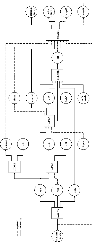 |
- case.scfX
- a file containing only the most significant output (see description below).
- plan.error
- error report file, should be empty later on successful completion of a program (meet chapter half dozen)
The following tables describe input and output files for the initialization programs nn , sgroup , symmetry , lstart , kgen , dstart (table 4.i), the utility programs tetra , irrep , spaghetti , aim , lapw7 , elnes , lapw3 , lapw5 , xspec , optic , joint , kram , optimize and mini (tabular array 4.2) as well as for a SCF bike of a non-spin-polarized example (table 4.two). Optional input and output files are used only if present in the respective case subdirectory or requested/generated past an input switch. The connection between FORTRAN units and filenames are defined in the corresponding programX.def files. The information flow is illustrated in Fig. 4.1.
| |||||||||||||||||||||||||||||||||||||||||||||||||||||||||||||||||||||||||||||||||||||||||||||||||||||||||||||||||||||||||||||
Input and output files of utility programs
| plan | needs | generates | ||
| necessary | optional | necessary | optional | |
| SPAGHETTI | spaghetti.def | case.qtl | example.spaghetti_ps | case.spaghetti_ene |
| instance.insp | case.outputso | instance.outputsp | ||
| case.struct | instance.irrep | instance.band.agr | ||
| instance.output1 | ||||
| TETRA | tetra.def | case.outputt | ||
| case.int | instance.dos1(2,3) | |||
| example.qtl | case.dos1ev(1,two,3) | |||
| example.kgen | ||||
| LAPW3 | lapw3.def | case.output3 | ||
| case.struct | case.rho | |||
| case.in2 | ||||
| case.clmsum | case.clmsum | |||
| LAPW5 | lapw5.def | case.sigma | case.output5 | case.rho.oned |
| case.struct | case.rho | |||
| instance.in5 | ||||
| instance.clmval | ||||
| XSPEC | xspec.def | case.outputx | case.coredens | |
| case.inc | example.dos1ev | |||
| case.int | example.xspec | |||
| example.vsp | case.txspec | |||
| instance.struct | case.m1 | |||
| case.qtl | case.m2 | |||
| OPTIC | optic.def | case.outputop | ||
| case.struct | case.symmat | |||
| instance.mat_diag | ||||
| instance.inop | ||||
| case.vsp | ||||
| case.vector | ||||
| Articulation | joint.def | case.outputjoint | case.sigma_intra | |
| case.injoint | case.joint | instance.intra | ||
| case.struct | ||||
| case.kgen | ||||
| case.weight | ||||
| instance.symmat | ||||
| example.mat_diag | ||||
| KRAM | kram.def | instance.epsilon | case.eloss | |
| case.inkram | case.sigmak | case.sumrules | ||
| case.joint | ||||
| OPTIMIZE | example.struct | case_initial.struct | optimize.job | case_vol_xxxxx.struct |
| case_c/a_xxxxx.struct | ||||
| MINI | mini.def | case.scf_mini | example.outputM | case.clmsum_inter |
| instance.inM | case.tmpM | instance.tmpM1 | ||
| case.finM | case.constraint | case.struct1 | ||
| case.scf | case.clmhist | case.scf_mini1 | ||
| case.struct | .min_hess | .minrestart | ||
| IRREP | case.struct | case.outputirrep | ||
| case.vector | case.irrep | |||
| AIM | instance.struct | case.outputaim | case.crit | |
| case.clmsum | case.surf | |||
| example.inaim | ||||
| LAPW7 | case.struct | instance.output7 | case.abc | |
| case.vector | example.grid | |||
| case.in7 | example.psink | |||
| case.vsp | ||||
| QTL | instance.struct | instance.outputq | ||
| case.vector | case.qtl | |||
| case.inq | ||||
| instance.vsp | ||||
Input and output files of chief programs in an SCF cycle
| program | needs | generates | ||
| necessary | optional | necessary | optional | |
| LAPW0 | lapw0.def | case.clmup/dn | example.output0 | case.r2v |
| instance.struct | case.vrespsum/up/dn | case.scf0 | case.vcoul | |
| case.in0 | case.inm | case.vsp(upwardly/dn) | case.vtotal | |
| case.clmsum | case.vns(upwardly/dn) | |||
| ORB | orb.def | example.energy | case.outputorb | case.br1orb |
| example.struct | case.vorb_old | case.scforb | case.br2orb | |
| case.inorb | case.vorb | |||
| case.dmat | orb.error | |||
| case.vsp | ||||
| LAPW1 | lapw1.def | case.vns | example.output1 | case.nsh(s) |
| case.struct | case.vorb | case.scf1 | example.nmat_only | |
| case.in1 | instance.vector.one-time | case.vector | ||
| case.vsp | case.free energy | |||
| case.klist | ||||
| LAPWSO | lapwso.def | case.vorb | case.vectorso | |
| case.struct | case.outputso | |||
| case.inso | case.scfso | |||
| instance.in1 | example.energyso | |||
| instance.vector | case.normso | |||
| case.vsp | ||||
| instance.vns | ||||
| case.energy | ||||
| LAPW2 | lapw2.def | instance.kgen | case.output2 | case.qtl |
| case.struct | case.nsh | case.scf2 | case.weight | |
| case.in2 | example.weight | case.clmval | case.weigh | |
| case.vector | case.counterbalance | case.help03* | ||
| instance.vsp | case.recprlist | case.vrespval | ||
| case.energy | case.almblm | |||
| instance.radwf | ||||
| LAPWDM | lapwdm.def | case.inso | example.outputdm | |
| case.struct | case.scfdm | |||
| example.indm | case.dmat | |||
| case.vector | lapwdm.error | |||
| case.vsp | ||||
| instance.weigh | ||||
| case.energy | ||||
| SUMPARA | case.struct | instance.scf2p | example.outputsum | |
| case.clmval | case.clmval | |||
| example.scf2 | ||||
| LCORE | lcore.def | case.vns | case.outputc | case.corewf |
| case.struct | instance.scfc | |||
| instance.inc | case.clmcor | |||
| example.vsp | lcore.fault | |||
| After LCORE the case.scfX files are appended to case.scf and the | ||||
| instance.clmsum file is renamed to example.clmsum_old (meet run_lapw ) | ||||
| MIXER | mixer.def | instance.clmsum_old | instance.outputm | case.broyd* |
| case.struct | case.clmsc | case.scfm | ||
| instance.inm | instance.clmcor | case.clmsum | ||
| instance.clmval | case.scf | mixer.mistake | ||
| case.broyd1 | ||||
| instance.broyd2 | ||||
| Later MIXER the file example.scfm is appended to case.scf , then that afterwards an iteration is | ||||
| completed, the two essential files are case.clmsum and case.scf . | ||||
two Clarification of general input/output files
In the following department the content of the (non-trivial) output files is described:
- case.almblm
- Contains the coefficients of the wavefunctions (generated optional by lapw2 ).
- case.broydX
- Contains the charge density of previous iterations if you utilize Broyden'southward method for mixing. They are removed when using save_lapw . They should exist removed by manus when calculational parameters (RKMAX, kmesh, ...) accept been inverse, or the calculation crashed due to a too large mixing and are restarted by using a new density generated by dstart.
- case.clmcor
- Contains the core charge density (as
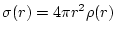 and has only a spherical part). In spin-polarized calculations 2 files example.clmcorup and case.clmcordn are used instead.
 - case.clmsc
- Contains the semi-core charge density in a 2-window calculation, which is no longer recommended. In spin-polarized calculations two files are used instead: instance.clmscup and case.clmscdn .
- case.clmsum
- Contains the total charge density in the lattice harmonics representation and equally Fourier coefficients. (The LM=0,0 term is given as , the others every bit
 ; suitable for generating electron density plots using lapw5 when the TOT-switch is ready, (see department 8.vi). In spin-polarized calculations two boosted files example.clmup and case.clmdn contain the spin densities. Generated by dstart or mixer .
 - case.clmval
- Contains the valence charge density as ; suitable for generating valence electron density plots using lapw5 when the VAL-switch is set, (see 8.6). In spin-polarized calculations two files case.clmvalup and example.clmvaldn are used instead.
- example.dmatup/dn
- Contains the density matrix generated by lapwdm for LDA+U, OP or Hybrid-DFT calculations.
- case.dosX
- Contains the density of states (states/Ry) and corresponding free energy (in Ry at the internal energy scale) generated by tetra . 10 tin exist 1-3. Additional files case.dosXev contain the DOS in (states/eV) and the energy in eV with respect to EF.
- case.help03X
- Contains eigenvalues and partial charges for atom number X.
- case.kgen
- This file contains the indices of the tetrahedra in terms of the list of one thousand-points. It is used in lapw2 (if EFMOD switch in instance.in2 is set to TETRA, encounter vii.v.3) and in tetra .
- case.klist
- This file contains a list of k-points in the offset BZ and represents a tetrahedral (special point) mesh. It is generated in kgen and tin either be inserted into the case.in1 file or used directly in kgen .
- case.qtl
- Contains eigenvalues and corresponding fractional charges (bandwise) in a form suitable for tetra and band structure plots with ``band character''. The decomposition of these charges is controlled past ISPLIT in case.struct.
- case.radwf
- Contains the radial basis functions inside spheres (generated optional by lapw2 ).
- case.rho
- Contains the electron densities on a filigree in a specified airplane generated by lapw5 . This file tin can exist used as input for your favorite contour or 3D plotting program.
- instance.rsp
- Contains the atomic densities generated by lstart . They are used by dstart to generate a offset crystalline density ( case.clmsum ).
- case.r2v
- Contains the commutation potential (in the lattice harmonics representation every bit
 and as Fourier coefficients) in a form suitable for plotting with lapw5 .
 - case.scf_mini
- Contains the last scf-iteration of each individual time (geometry) stride during a structural minimization using mini . Thus this file contains a complete history of properties (energy, forces, positions) during a structural minimization.
- case.sigma
- Contains the atomic densities for those states with a ``P'' in case.inst . Generated in lstart and used for difference densities in lapw5 .
- example.spaghetti_ps
- A ps file with the energy bandstructure plot generated by spaghetti .
- case.band.agr
- A xmgrace file with the energy bandstructure plot generated by spaghetti .
- case.vcoul
- Contains the Coulomb potential (in the lattice harmonics representation as and as Fourier coefficients) in a form suitable for plotting with lapw5 .
- example.vorb
- Contains the orbital potential (in Ry) generated past orb for LDA+U or hybrid-DFT calculations in grade of a (2l+1,2l+one) matrix.
- case.vtotal
- Contains the full potential (in the lattice harmonics representation as and every bit Fourier coefficients) in a class suitable for plotting with lapw5 .
- case.vector
- Binary file, contains the eigenvalues and eigenvectors of all k-points calculated in lapw1 . In spin-polarized calculations two files instance.vectorup and case.vectordn are used instead. lapwso generates case.vectorso .
- case.energy
- Contains the eigenvalues of all k-points calculated in lapw1 . In spin-polarized calculations 2 files example.vectorup and case.vectordn are used instead. lapwso generates example.energyso .
- case.vns
- Contains the non-spherical part of the total potential Five. Inside the sphere the radial coefficients of the lattice harmonics representation are listed (for L greater than 0), while for the interstitial region the reanalyzed Fourier coefficients are given (run across equ. (2.10)). In spin-polarized calculations 2 files instance.vnsup and case.vnsdn are used instead.
- case.vorbup/dn
- Contains the orbital dependent function of the potential in LDA+U, OP or Hybrid-DFT calculations. Generated in orb , used in lapw1 .
- case.vsp
- Contains the spherical part of the total potential 5 stored as
 (thus the first values should be shut to
  ). In spin-polarized calculations two files case.vspup and case.vspdn are used instead.
three The ``master input`` file case.struct
The file case.struct defines the structure and is the principal input file used in all programs. We provide several examples in the subdirectory
example_struct_file
If you are using the ``Struct Generator'' from the graphical user interface w2web, you don't accept to bother with this file direct! Yet, the description of the fields of the input mask can be found here.
Annotation: If yous are changing this file manually, please note that this is a formatted file and the proper cavalcade positions of the characters are of import! Use REPLACE instead of DELETE and INSERT during edit!
We commencement the clarification of this file with an abridged example for rutile TiO (calculation line numbers):
--------------------- top of file ---------------------line # Titaniumdioxide TiO2 (rutile): u=0.305 1 P LATTICE,NONEQUIV. ATOMS ii 2 Mode OF CALC=RELA 3 8.6817500 8.6817500 v.5916100 ninety. xc. 90. 4 Cantlet -i: X= 0.0000000 Y= 0.0000000 Z= 0.0000000 5 MULT= two ISPLIT= 8 6 Cantlet -1: X= 0.5000000 Y= 0.5000000 Z= 0.5000000 Titanium NPT= 781 R0=.000022391 RMT=2.00000000 Z:22.0 7 LOCAL ROT MATRIX: -.7071068 0.7071068 0.0000000 viii 0.7071068 0.7071068 0.0000000 9 0.0000000 0.0000000 one.0000000 10 Cantlet -two: X= 0.3050000 Y= 0.3050000 Z= 0.0000000 MULT= 4 ISPLIT= 8 Cantlet -2: X= 0.6950000 Y= 0.6950000 Z= 0.0000000 ATOM -ii: X= 0.8050000 Y= 0.1950000 Z= 0.5000000 ATOM -two: X= 0.1950000 Y= 0.8050000 Z= 0.5000000 Oxygen NPT= 781 R0=.000017913 RMT=1.60000000 Z: 8.0 LOCAL ROT MATRIX: 0.0000000 -.7071068 0.7071068 0.0000000 0.7071068 0.7071068 1.0000000 0.0000000 0.0000000 16 SYMMETRY OPERATIONS: 11 1 0 0 0.00 12 0 1 0 0.00 thirteen 0 0 1 0.00 xiv 1 15 1 0 0 0.00 0 1 0 0.00 0 0-one 0.00 2 ........ xv 0 i 0 0.50 -ane 0 0 0.fifty 0 0 1 0.l sixteen ------------------ lesser of file ---------------------------
Interpretive comments on this file are as follows.
|
 ) sin(
 ), a cos(
 /ii, -a/2, c/3],[a/
- line 1:
- format (A80)
championship (chemical compound) - line ii:
- format (A4,23X,I3)
lattice blazon, NAT
lattice type every bit divers in table 4.4. For definitions of the triclinic lattice encounter SRC_nn/dirlat.f NAT number of inequivalent atoms in the unit prison cell - line 3:
- format (13X,A4)
mode
RELA fully relativistic core and scalar relativistic valence NREL non-relativistic adding - line 4:
- format (6F10.6)
a, b, c,
a, b, c unit jail cell parameters (in a.u., 1 a.u. = 0.529177 Å). In face- or body-centered structures the non-primitive (cubic) lattice constant, for rhombohedral (R) lattices the hexagonal lattice constants must be specified. (The following may help you to convert betwixt hexagonal and rhombohedral specifications: 
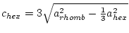
and (for fcc-like lattices) 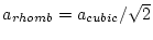
angles between unit centrality (if omitted,  is set equally default). Prepare it only for P and CXZ lattices
 - line 5:
- format (4X,I4,4X,F10.8,3X,F10.8,3X,F10.8)
cantlet-index, x, y, z
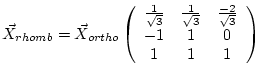
atom-index running index for inequivalent atoms positive in instance of cubic symmetry negative for not-cubic symmetry this is fix automatically using symmetry ten,y,z position of atom in internal units, i.e. as positive fractions of unit jail cell parameters. (  ; the positions in the unit of measurement prison cell are consistent with the convention used in the International Tables of Crystallography 64. In face- (body-) centered structures only one of four (two) atoms must be given, eg. in Fm3m position 8c is specified with 0.25, 0.25, 0.25 and .75, 0.75, 0.75). For R lattice utilise rhombohedral coordinates. (To catechumen from hexagonal into rhombohedral coordinates use the auxiliary program hex2rhomb , which can be called at a command-line: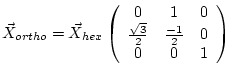
- line vi:
- format (15X,I2,17X,I2)
multiplicity, isplit
multiplicity number of equivalent atoms of this kind isplit this is just an output-option and is used to specify the decomposition of the lm-similar charges into irreducible representations, useful for interpretation in instance.qtl). This parameter is automatically set past symmetry : 0 no split of l-like accuse 1 p-z, (p-x, p-y) e.m.:hcp 2 e-grand, t-2g of d-electrons e.k.:cubic 3 d-z2, (d-xy,d-x2y2), (d-xz,dyz) due east.1000.:hcp 4 combining option i and iii e.k.:hcp 5 all d symmetries separate six all p symmetries separate 8 combining pick 5 and 6 -two d-z2, d-x2y2, d-xy, (d-xz,d-yz) 88 carve up  like charges (for telnes )
99 summate cross-terms (for telnes ) -
 : line 5
 - must now exist repeated MULT-1 times for the other positions of each equivalent atom according to the Wyckoff position in the ``International Tables of Crystallography''.
- line vii:
- format (A10,5X,I5,5X,F10.8,5X,F10.5,5X,F5.2)
proper name of atom, NPT, R0, RMT, Z
name of cantlet Use the chemical symbol. Positions iii-10 for further labeling of nonequivalent atoms (use a number in position 3) NPT number of radial mesh points (381 gives a good mesh for LDA calculations, but for GGA twice as many points are recommended; always use an odd number of mesh points!) the radial mesh is given on a logarithmic calibration: ![$r(n)=R_0 * e^{[ (n-1)*DX ]}$](https://euler.phys.cmu.edu/cluster/WIEN2k/img120.png)
R0 beginning radial mesh point (typically between 0.0005 and 0.00005, smaller for heavy elements, bigger for light ones; a struct-file generated by w2web will accept proper R0 values.) RMT atomic sphere radius (muffin-tin radius), can easily exist estimated after running nn (see 6.1) and are set automatically with setrmt_lapw run across five.two.half dozen). The following guidelines will exist given here: Choose spheres every bit large as possible every bit this will save MUCH reckoner fourth dimension. Simply: Use identical radii inside a serial of calculations (i.e. when you want to compare total energies) -- therefore consider outset how close the atoms may possibly come later on (book or geometry optimization); exercise NOT make the spheres as well different (fifty-fifty when the geometry would permit information technology), instead utilize the largest spheres for f-electron atoms, x-20 % smaller ones for d-elements and once again ten-20 % smaller for sp-elements; H is a special instance, you may choose it much smaller (e.chiliad. 0.6 and 1.ii for H and C) and systems containing H need a much smaller RKMAX value (3-5) in case.in1 . Z atomic number - line 8-10:
- format (20X,3F10.7)
ROTLOC local rotation matrix (always in an orthogonal coordinate system). Transforms the global coordinate arrangement (of the unit prison cell) into the local at the given atomic site equally required past bespeak group symmetry (see in the INPUT-Section 7.5.iii of LAPW2). SYMMETRY calculates the signal grouping symmetry and determines ROTLOC automatically. Note, that a proper ROTLOC is required, if the LM values generated by SYMMETRY are used. A more detailed description with several examples is given in the appendix A and sec. x.three - : lines 5 thru 10
- must be repeated for each inequivalent atom
- line 11:
- format (I4)
nsym number of symmetry operations of space group (encounter International Tables of Crystallography 64) If nsym is fix to zero, the symmetry operations volition exist generated automatically by SYMMETRY. - line 12-xiv:
- format (3I2,F10.vii)
matrix, tau (as listed in the International Tables of Crystallography 64)
matrix matrix representation of (infinite group) symmetry operation tau not-primitive translation vector - line fifteen:
- format (I8)
index of symmetry operation specified in a higher place
- : lines 12 thru 15
- must be repeated for all other symmetry operations
(the complete list is contained in sample inputs)
four The ``history`` file case.scf
During the self-consequent field (SCF) bicycle the essential data are appended to the file case.scf in society to generate a summary of previous iterations. For an easier retrieval of certain quantities the essential lines are labeled with :LABEL:, which tin can be used to monitor these quantities during self-consistency as explained below. The most important :LABELs are
| :ENE | total free energy (Ry) |
| :DIS | charge altitude betwixt last 2 iterations ( 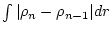 ). Good convergence criterium. ). Good convergence criterium. |
| :FER | Fermi energy |
| :FORxx | strength on atom 20 in mRy/bohr (in the local (for each atom) carthesian coordinate organisation) |
| :FGLxx | force on atom xx in mRy/bohr (in the global coordinate arrangement of the unit of measurement cell (in the aforementioned way equally the diminutive positions are specified)) |
| :DTOxx | total departure charge density for atom xx between last 2 iterations |
| :CTOxx | total charge in sphere twenty (mixed after MIXER) |
| :NTOxx | total accuse in sphere twenty (new (not mixed) from LAPW2+LCORE) |
| :QTLxx | partial charges in sphere xx |
| :EPLxx | 50-similar fractional charges and ``mean energies'' in lower (semicore) free energy window for atom xx. Used equally energy parameters in instance.in1 for next iteration |
| :EPHxx | l-like fractional charges and ``mean energies'' in higher (valence) free energy window for cantlet xx. Used as free energy parameters in example.in1 for adjacent iteration |
| :EFGxx | Electric field gradient (EFG)  for cantlet twenty for cantlet twenty |
| :ETAxx | Asymmetry parameter of EFG for atom xx |
| :RTOxx | Density for cantlet xx at the nucleus (start radial mesh indicate) |
| :VZERO | Gives the total, Coulomb and xc-potential at z=0 and z=0.5 (meaningfull just for slab calculations) |
To check to which blazon of calculation a scf file corresponds utilize:
| :POT | Exchange-correlation potential used in this calculation |
| :LAT | Lattice parameters in this adding |
| :VOL | Volume of the unit cell |
| :POSxx | Diminutive positions for cantlet xx (every bit in instance.struct ) |
| :RKM | Actual matrix size and resulting RKmax |
| :NEC | normalization check of electronic charge densities. If a meaning amount of electrons is missing, i might accept cadre states, whose charge density is not completely confined inside the respective diminutive sphere. In such a case the corresponding states should exist treated as ring states (using LOs). |
For spin-polarized calculations:
| :MMTOT | Full spin magnetic moment/cell |
| :MMIxx | Spin magnetic moment of cantlet twenty. Notation, that this value depends on RMT. |
| :CUPxx | spin-upward accuse (mixed) in sphere xx |
| :CDNxx | spin-dn charge (mixed) in sphere twenty |
| :NUPxx | spin-up charge (new, from lapw2+lcore) in sphere xx |
| :NDNxx | spin-dn charge (new, from lapw2+lcore) in sphere twenty |
| :ORBxx | Orbital magnetic moment of atom twenty (needs SO calculations and LAPWDM). |
| :HFFxx | Hyperfine field of atom twenty (in kGauss). |
One tin can monitor the energy eigenvalues (listed for the showtime k-point merely), the Fermi-energy or the total energy. Often the electronic charges per cantlet reflect the convergence. Charge transfer between the various diminutive spheres is a typical process during the SCF cycles: large oscillations should exist avoided past using a smaller mixing parameter; monotonic changes in one direction advise a larger mixing parameter.
In spin-polarized calculations the magnetic moment per atomic site is an additional crucial quantity which could exist used as convergence criterion.
If a system has electric field gradients and ane is interested in that quantity, one should monitor the EFGs, because these are very sensitive quantities.
Information technology is best to monitor several quantities, because often one quantity is converged, while some other still changes from iteration to iteration. The script run_lapw has 3 dissimilar convergence criteria built in, namely the total free energy, the atomic forces and the charge distance (come across 5.1.2, 5.ane.3).
Nosotros recommend the use of UNIX commands like :
grep :ENE case.scf or use ``Assay'' from w2web
for monitoring such quantities.
Y'all may ascertain an allonym for this (see sec. 11.2), and a csh-script grepline_lapw is also available to become a quantity from several scf-files simultaneously (sec. five.2.16 and 5.3).
5 Flow of programs
The WIEN2k packet consists of several independent programs which are linked via C-Vanquish SCRIPTS described below.
The flow and usage of the different programs is illustrated in the following diagram (Fig. 4.2):
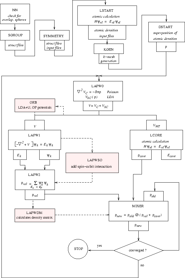 |
The initialization consists of running a series of small auxiliary programs, which generates the inputs for the principal programs. Ane starts in the respective example/ subdirectory and defines the structure in instance.struct (see iv.three). The initialization can exist invoked by the script init_lapw (encounter sec. iii.7 and 5.1.ii), and consists of running:
- NN
- a plan which lists the nearest neighbor distances upwards to a specified limit (divers past a distance factor f) and thus helps to determine the atomic sphere radii. In addition it is a very usefull additional cheque of your case.struct file (equivalency of atoms)
- SGROUP
- determines the spacegroup of the structure defined in your case.struct file.
- SYMMETRY
- generates from a raw example.struct file the infinite group symmetry operations, determines the bespeak group of the individual atomic sites, generates the LM expansion for the lattice harmonics and determines the local rotation matrices.
- LSTART
- generates free diminutive densities and determines how the different orbitals are treated in the band construction calculations (i.e. as core or band states, with or without local orbitals,...).
- KGEN
- generates a k-mesh in the irreducible part of the BZ.
- DSTART
- generates a starting density for the scf wheel by a superposition of diminutive densities generated in LSTART.
So a self-consistency bike is initiated and repeated until convergence criteria are met (see 3.8 and 5.1.3). This bicycle tin be invoked with a script run_lapw , and consists of the following steps:
- LAPW0
- (POTENTIAL) generates potential from density
- LAPW1
- (BANDS) calculates valence bands (eigenvalues and eigenvectors)
- LAPW2
- (RHO) computes valence densities from eigenvectors
- LCORE
- computes cadre states and densities
- MIXER
- mixes input and output densities
1 Core, semi-core and valence states
In many cases information technology is desirable to distinguish iii types of electronic states, namely core, semi-core and valence states. For instance titanium has core ( ,
,  ,
,  ), semi-core (
 ,
,  ) and valence (
 ,
,  ,
,  ) states. In our definition cadre states are only those whose charge is entirely confined within the corresponding atomic sphere. They are deep in free energy, east.g., more than vii-x Ry below the Fermi energy. Semi-core states prevarication high enough in energy (between nigh i and 7 Ry below the Fermi free energy), so that their charge is no longer completely confined inside the diminutive sphere, simply has a few per centum outside the sphere. Valence states are energetically the highest (occupied) states and ever accept a significant amount of charge exterior the spheres.
The energy cut-off specified in lstart during init_lapw (unremarkably -6.0 Ry) defines the separation into core- and band-states (the latter incorporate both, semicore and valence). If a system has atoms with semi-cadre states, and so the all-time way to care for them is with ``local orbitals``, an extension of the usual LAPW basis. An input for such a basis set will be generated automatically. (Additional LOs can also be used for valence states which have a strong variation of their radial wavefunctions with energy (e.m. d states in TM compounds) to improve the quality of the basis set up, i.east. to go beyond the simple linearization).
two Spin-polarized calculation
For magnetic systems spin-polarized calculations can exist performed. In such a case some steps are washed for spin-up and spin-down electrons separately and the script runsp_lapw consists of the following steps:
- LAPW0
- (POTENTIAL) generates potential from density
- LAPW1 -up
- (BANDS) calculates valence bands for spin-upwards electrons
- LAPW1 -dn
- (BANDS) calculates valence bands for spin-downward electrons
- LAPW2 -upward
- (RHO) computes valence densities for spin-upwards electrons
- LAPW2 -dn
- (RHO) computes valence densities for spin-down electrons
- LCORE -up
- computes core states and densities for spin-up electrons
- LCORE -dn
- computes cadre states and densities for spin-downwards electrons
- MIXER
- mixes input and output densities
The use of spin-polarized calculations is illustrated for fcc Ni (section 10.2), one of the test cases provided in the WIEN2k package.
3 Fixed-spin-moment (FSM) calculations
Using the script runfsm_lapw -k 20 it is possible to constrain the total spin magnetic moment per unit cell to a fixed value 20 and thus force a particular ferromagnetic solution (which may non correspond to the equillibrium). This is specially useful for systems with several metastable (non-) magnetic solutions, where conventional spin-polarized calculation would not converge or the solution may depend on the starting density. Additional SO-interaction is not supported.
Delight note, that once runfsm_lapw has finished, but example.vectordn is ok, but instance.vectorup is NOT the proper up-spin vector and MUST Non be used for the calculations of QTLs (and DOS). It must be regenerated by x lapw1 -up (meet also the comments for iterative diagonalization in section 5.two.18).
4 Antiferromagnetic (AFM) calculations
Several considerations are necessary, when you want to perform an AFM calculation. Please have also a look into $WIENROOT/SRC_afminput/afminput_test.
- You must construct a unit of measurement jail cell which allows for the desired AF ordering. For case for bcc Cr you must select a ``P'' lattice and specify both atoms, Cr1 at (0,0,0) and Cr2 at (.5,.5,.5), respective to a CsCl structure. Note, that it is important to label the 2 Cr atoms with ``Cr1'' and ``Cr2'', since only then the symmetry programs can detect that those atoms should be different (although they take the same Z). If sgroup has interchanged some axis, endeavor to disengage these changes, since afminput may not properly find the right symmetry operations in such a case.
- When you lot generate instance.inst you must specify the correct magnetic gild and flip the spin of the AF atoms (i.e. invert the spin upwardly and dn occupation numbers). In improver you lot should set a nil moment (identical spin up and dn occupations) for all ``non-magnetic'' atoms. This can exist done conveniently using instgen_lapw -ask or during ``initialization'' using w2web.
- Now yous can run either a ``normal'' spinpolarized initialization (without AFM option) and runsp_lapw or:
- Create a struct file of the non-magnetic (or ferro-magnetic) supergroup (run init_lapw upwards to lstart). Name it example.struct_supergroup . (For example for bcc Cr, this would exist a struct file with the ordinary cubic lattice parameters, ``B'' blazon lattice and just i Cr at (0,0,0).)
- Run init_lapw . At the end AFMINPUT creates an input file for the program CLMCOPY. Depending on the presence of case.struct_supergroup and the specific symmetry it may/may non ask you to supply a symmetry operation/nonprimitive translation (meet Sect. 9.v .
- Run runafm_lapw . This script calls LAPW1 and LAPW2 only for spin-upward but the corresponding spin-dn density is created by CLMCOPY according to the rules defined during initialization. This reduces the required cpu fourth dimension by a factor of two (and in addition the scf cycle is much more stable).
- It is highly recommended that you save your work ( save_lapw ) and check the results by continuing with a regular runsp_lapw . If zip changes (E-tot and other properties), and then you are ok, otherwise make sure the scf calculation is well converged (-cc 0.0001 or better). Eventually the system may not want to be antiferromagnetic (but for instance it is ferrimagnetic!).
runafm_lapw saves you more a factor of ii in in calculator time, since only spin-upwards is calculated and in addition the scf-convergence may be MUCH faster. It works also with LDA+U ( case.dmatup/dn are also copied), but does Non work with Hybrid-DFT nor spin-orbit coupling, since this requires the presence of both vector files in the LAPWSO pace.
5 Spin-orbit interaction
You can add spin-orbit interaction in LAPWSO (called directly afterwards LAPW1) using a 2nd-variational method with the scalar-relativistic orbitals (from LAPW1) as basis. The number of eigenvalues will double since SO couples spin-up and dn states, so they are no longer separable. In addition, LOs with a `` '' radial ground tin can exist added. (Kunes et al. 2001)
To aid with the generation of the necessary input files and possible changes in symmetry, a script initso_lapw exists. For non-spinpolarized cases nothing item must be taken into account so tin be hands applied by running run_lapw -so . It will automatically apply the circuitous version of LAPW2.
However, for spin-polarized cases, the And then interaction may alter (lower) the symmetry depending on how you choose the direction of magnetization and care must be taken to become a proper setup. initso_lapw together with symmetso generates the proper symmetry.
Simply a few hints what can happen:
- Suppose y'all have a cubic organization and put the magnetization forth [001]. This will create a tetragonal symmetry (and you can temporarely tell this to the initialization programs by changing the respective lattice parameter c to a tetragonal system).
- If yous put the magnetization forth [111], this creates most likely a rhombohedral (or hexagonal) symmetry. (Try to visualize this for a fcc lattice, XCRYSDEN is very usefull for this purpose).
- Symmetry operations tin exist classified into operations which capsize the magnetization,others which leave it unchanged and some which practise some arbitrary rotation. The program symmetso (part of initso_lapw ) sorts these operations in the proper way.
- If you don't accept inversion symmetry in the original structure, you must non ``add together inversion'' in KGEN.
The recommended style to include And then in the calculations is to run a regular scf calculation first, save the results, initialize SO and run some other scf cycle including SO:
- run[sp]_lapw
- save_lapw case_nrel
- initso_lapw
- run[sp]_lapw -so
For spin-polarized systems yous may want to add the ``-dm'' switch to summate also the orbital magnetic moment.
six Orbital potentials
In WIEN2kit is possible to become beyond standard LDA (GGA) and include orbital dependent potentials in methods like LDA+U or the ''Orbital-Polarization'', which are very usefull for strongly correlated systems. To use these features yous need to create input-files for LAPWDM and ORB ( case.indm, case.inorb ). Y'all may copy a template from SRC_templates , but must modify information technology according to your needs. In particular you must select for which atoms and which orbitals (usually d-Orbitals of late transition metal atoms or f-orbitals for 4f/5f atoms) y'all want to add such a potential and as well choose the proper U and J values for them. Once this is washed, you can include this using the -orb switch. The density matrix ( case.dmatup/dn ) will be calculated after lapw2 in lapwdm , it will be mixed in mixer (consistently with the ``regular'' accuse density) and the orbital dependend potentials will be calculated on orb (after lapw0 ). Note, you must run spin-polarized in club to utilize orbital potentials.
- runsp_lapw -orb [-so]
If yous desire to strength a non-magnetic solution you can constrain the spin-polarization to zero using runsp_c_lapw .
Without And then, case.vorbup/dn volition exist considered in LAPW1(c). With So, it will be practical in LAPWSO (and allows coupling of nondiagonal spin-terms).
7 Verbal-exchange and Hybrid functionals for correlated electrons
In WIEN2kinformation technology is also possible to become beyond standard LDA (GGA) and include on-site exact-exchange (Hartree-Fock), which is very usefull for strongly correlated systems. The exact-exchange/hybrid methods are implemented only within the atomic spheres, therefore it is recommended to us them just for localized electrons (see Tran et al. 2006 for details). They will NOT improve gaps in sp-semiconductors. Examples of implemented functionals include:
- LDA-Hartree-Fock
Functional five in instance.in0. way = EECE and fraction = i in case.ineece.![\begin{displaymath} E_{xc}^{\textrm{LDA-HF}}[\rho] = E_{xc}^{\textrm{LDA}}[\rho]... ...{\textrm{corr}}] - E_{xc}^{\textrm{LDA}}[\rho_{\textrm{corr}}] \end{displaymath}](https://euler.phys.cmu.edu/cluster/WIEN2k/img124.png)
- LDA-Fock-

Functional 5 in example.in0. style = HYBR and fraction = in example.ineece. ![\begin{displaymath} E_{xc}^{{\textrm{LDA-Fock-}}\alpha}[\rho] = E_{xc}^{\textrm{... ...rm{corr}}] - E_{x}^{\textrm{LDA}}[\rho_{\textrm{corr}}]\right) \end{displaymath}](https://euler.phys.cmu.edu/cluster/WIEN2k/img125.png)
- PBE-Fock-
Functional thirteen in case.in0. mode = HYBR and fraction = in example.ineece. ![\begin{displaymath} E_{xc}^{\textrm{PBE-Fock-}\alpha}[\rho] = E_{xc}^{\textrm{PB... ...rm{corr}}] - E_{x}^{\textrm{PBE}}[\rho_{\textrm{corr}}]\right) \end{displaymath}](https://euler.phys.cmu.edu/cluster/WIEN2k/img126.png)
The PBE0 functional corresponds to .
. - PBEsol-Fock-
Functional 19 in instance.in0. mode = HYBR and fraction = in case.ineece.
- WC-Fock-
Functional xi in case.in0. mode = HYBR and fraction = in example.ineece.
- TPSS-H-Fock-
Functional 27 in case.in0. way = HYBR and fraction = in case.ineece.
It is similar to PBE0, just uses the meta-GGA TPSS. - B3PW91
Functional 18 in example.in0. mode = HYBR and fraction = 0.2 in example.ineece.![\begin{eqnarray*} E_{xc}^{\textrm{B3PW91}}[\rho] & = & E_{xc}^{\textrm{LDA}}[\rh... ...(E_{c}^{\textrm{PW91}}[\rho] - E_{c}^{\textrm{LDA}}[\rho]\right) \end{eqnarray*}](https://euler.phys.cmu.edu/cluster/WIEN2k/img131.png)
In addition to the input files which are necessary for an usual LDA or GGA adding, the input file case.ineece is necessary to start a calculation. You may copy a template from SRC_templates , but must change information technology according to your needs. In particular you must select for which atoms and which orbitals (commonly d-Orbitals of late transition metal atoms or f-orbitals for 4f/5f atoms) yous want to add such a potential and which blazon of functional you want to utilize.
A sample input for calculations with exact exchange is given below.
------------------ top of file: case.ineece ----------- -9.0 2 emin, natorb 1 one 2 1st atom index, nlorb, lorb 2 one 2 2nd atom index, nlorb, lorb HYBR HYBR / EECE mode 0.25 fraction of exact exchange ------------------ bottom of file ---------------------
Interpretive comments on this file are as follows:
line 1: complimentary format
emin, natom
| emin | lower free energy cutoff, to be selected so that the free energy of correlated states is larger than emin | |
| natorb | number of atoms for which the verbal exchange is calculated |
iatom(i), nlorb(i), (lorb(li,i), li=1,nlorb(i))
| iatom | index of cantlet in struct file | |
| nlorb | number of orbital moments for which exact exchange shall be calculated | |
| lorb | orbital numbers (repeated nlorb-times) |
 line repeated natorb-times
 line 3: gratis format
mode
| HYBR | means that LDA/GGA exchange will be replaced by exact exchange | |
| EECE | means that LDA/GGA exchange-correlation volition be replaced by verbal commutation |
| alpha | This is the fraction of Hartree-Fock exchange (between 0 and 1) |
Every bit with LDA+ , hybrid functionals can be used only for spin-polarized calculations ( runsp_lapw with the switch -eece ). runsp_lapw volition internally phone call runeece_lapw , which will create all necessary additional input files (it requires a case.in0 file including the optional IFFT line as generated by init_lapw ): example.indm (example.indmc), case.inorb, case.in0eece, case.in2eece (case.in2ceece) and once this is washed, calculates in a series of lapw2/lapwdm/lapw0/orb calculations the corresponding orbital dependend potentials.
- runsp_lapw -eece [-so]
8 modified Becke-Johnson potential (mBJ) for band gaps
The modified Becke-Johnson exchange potential + LDA-correlation (Tran and Blaha 2009) allows the adding of band gaps with an accuracy similar to very expensive GW calculations. It is a local approximation to an diminutive ``verbal-substitution''-potential and a screening term. This is just a 90-potential, not a 90-free energy functional, thus  is taken from LSDA and the forces cannot be used with this option.
We recommend the following steps to perform such calculations:
- run a regular initialization and scf cycle using LDA or PBE,
- create instance.inm_vresp ( cp $WIENROOT/SRC_templates/case.inm_vresp case.inm_vresp .
- edit case.in0 and set "R2V" selection (instead of "NR2V").
- run one more scf-wheel (utilize run_lapw -NI -i i ) to generate the required instance.vresp* files.
- ``save'' the LDA (PBE) calculation.
- edit case.in0 and change the functional to option indxc=28.
- cp case.in0 example.in0_grr and modify indxc in case.in0_grr to 50. This pick will calculate the average of over the unit of measurement cell. (The presence of case.in0_grr will exist detected during the scf-wheel and lapw0 will be called twice, first with the input file instance.in0_grr , then with instance.in0 .)
- run another scf cycle.
In most cases MSEC1 mixing volition lead to convergence issues of the scf bike. One should switch in example.inm to PRATT mixing, showtime using a smaller mixing factor (eg. 0.2), later increasing it to 0.50.
Next: 5 Shell scripts Up: 2 Detailed description of Previous: two Detailed clarification of Contents pblaha 2011-03-22
Source: https://euler.phys.cmu.edu/cluster/WIEN2k/4Files_Program.html
0 Response to "When I Delet File From Wien2k and I Want to Login Againe"
Postar um comentário